Memory: Allocation Schemes and Relocatable Code

Posted 4/26/20

This Spring I’m a graduate teaching assistant for an operating systems course. Campus is closed during the COVID-19 epidemic, so I’ve been holding office hours remotely and writing up a range of OS explanations. Below is one of these writeups for a recent topic of some confusion.

There are, broadly, four categories of memory allocation schemes that operating systems use to provision space for executables. This post will discuss each of them in historical order, with pros and cons, and some executable formats (relocatable and position-independent code) that are closely intertwined. We’ll include shared memory and dynamic libraries at the end. Note that we are not talking about malloc and free - the way an application allocates and deallocates memory within the space the operating system has already assigned it - but the way the operating system assigns memory to each program.

1: Flat Memory Model / Single Contiguous Allocation

In a flat memory model, all memory is accessible in a single continuous space from 0x0 to the total bytes of memory available in the hardware. There is no allocation or deallocation, only total access to all available memory. This is appropriate for older computers that only run one program at a time, like the Apple II or Commodore 64. If a program needs to keep track of which memory it’s used then it may implement a heap and something like malloc and free within the memory range. However, if we want to run multiple programs at the same time then we have a dilemma. We want each program to have its own memory for variables, without stepping on one another. If both programs have full access to all the memory of the system then they can easily and frequently write to the same memory addresses and crash one another.

2: Fixed Contiguous Memory Model

Enter our second model, designed explicitly for multi-process systems. In this model, memory is broken into fixed-length partitions, and a range of partitions can be allocated to a particular program. For example, the following is a diagram of memory broken into 40 equally-sized blocks, with three programs (marked A, B, and C) running:

AAAAAAAAAA
AA........
..BBBBBBB.
...CCCCC..

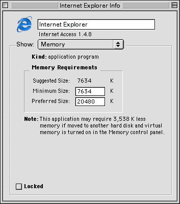
When a program starts, the operating system determines how much memory it will need for static variables and the estimated stack and heap sizes. This is usually a guess based on the size of the executable file plus some wiggle room, but in older operating systems you could often override the system’s guess if you knew the executable required more memory:

Once the operating system determines how much memory is needed, it rounds up to the nearest partition size and determines how many blocks are required. Then it looks for an area of unallocated memory large enough to fit the executable (using one of the algorithms described below), assigns those blocks to the executable, and informs the executable of where its memory begins (a base address) and how much memory it can use.

Since we can only assign an integer number of blocks, there is always some waste involved: A program requiring 1.1 blocks of space will be assigned 2 blocks, wasting most of a block. This is called internal fragmentation.

First-Fit

In the simplest algorithm, the operating system scans memory for the first open space large enough to fit the new program. This is relatively quick, but often leads to poor choices, such as in the following scenario:

AAAAAAAAAA
AA........
..BBBBBBB.
...CCCCC..

We have a new program ‘D’ that we want to start running, which requires three blocks worth of memory. In a First-Fit algorithm we might place ‘D’ here:

AAAAAAAAAA
AADDD.....
..BBBBBBB.
...CCCCC..

This suits D’s purposes perfectly, but means we have reduced the largest free memory space available, so we can no longer fit programs larger than 7 blocks in length.

Next-Fit

The first-fit algorithm also uses memory unevenly - since it always searches memory from 0x0 onwards, it will prefer placing programs towards the start of memory, which will make future allocations slower as it scans over a larger number of assigned blocks. If we keep track of the last assigned block and search for new blocks from that point, the algorithm is called next-fit, and is a slight optimization over first-fit.

Best-Fit

In the “Best-Fit” algorithm we scan all of memory for the smallest unallocated space large enough to fit the program. In this case we would allocate ‘D’ here:

AAAAAAAAAA
AA........
..BBBBBBBD
DD.CCCCC..

This is better in the sense that we can still fit programs of 10 blocks in size, but there’s a downside: The space immediately after ‘D’ is only one block long. Unless the user starts a very small 1-block executable, this space will be effectively useless until either process ‘D’ or ‘C’ exits. Over time, the best-fit algorithm will create many-such holes. If there is sufficient total space for a program, but no unallocated region is large enough to load it, we use the term external fragmentation.

Worst-Fit

“Worst-Fit” is something of a misnomer and should be thought of as “the opposite of best-fit”. In worst-fit we find the largest unallocated memory space, and assign the first blocks from this region to the new program. This avoids the external fragmentation problems of the best-fit algorithm, but encounters the same problem as our first-fit example: A larger program will not have space to run, because we’ve been nibbling away at all the largest memory regions.

Relocatable Code

In order to implement any of these memory allocation schemes, we must be able to tell programs where their variables may be placed. Traditional flat-memory executables use absolute addressing, meaning they refer to variable locations by hard-coded memory addresses. In order to run multiple processes concurrently we need to redesign the executable format slightly to use some kind of offset table. When the program starts, the operating system fills in the true locations of variables in this table, and programs refer to variable locations by looking them up in this table rather than hardcoding the absolute variable locations in. This ability to have executable code run at any starting address in memory is called relocatable code. The exact implementation details of relocation are platform-specific.

As a side-note, we also use relocatable code during the compilation of executables. Object files (.o files) are parts of a program that have been compiled, but not yet linked to one another to create the final executable. Because of this, the final locations of variables are not yet known. The linker fills out the variable locations as it combines the object files.

Defragmentation

Obviously when a program exits we can reclaim the memory it used. Why can’t we move executables while they’re running? Specifically, why can’t we go from:

AAAAAAAAAA
AA........
..BBBBBBBD
DD.CCCCC..

To a cleaner:

AAAAAAAAAA
AABBBBBBBD
DDCCCCC...
..........

This would give us all the room we need for large executables! Unfortunately even relocatable executables aren’t this flexible - while they are designed to be started at any memory location, once the program is running it may create pointers to existing variables and functions, and those pointers may use absolute memory addresses. If we paused an executable, moved it, rewrote the relocation table, and resumed it, then many pointers would be invalid and the program would crash. There are ways to overcome these limitations, but when we get to virtual memory the problem goes away on its own.

3: Dynamic Contiguous Memory Model

The dynamic contiguous memory model is exactly the same as the fixed contiguous memory model, except that blocks have no fixed, pre-determined size. We can assign an arbitrary number of bytes to each executable, eliminating internal fragmentation. This adds significant overhead to the operating system, but from an application perspective the executable is similarly given a starting position and maximum amount of space.

4: Virtual Memory

The modern approach to memory allocation is called virtual memory. In this system we create two separate addressing modes: logical addresses, which are seen by the executable, and physical addresses, which are the true locations of variables seen by the operating system. Whenever the executable reads or writes any memory the operating system translates between the userspace logical address and the physical memory address.

Adding a translation layer before every memory access adds massive overhead - after all, programs read and write to variables all the time! However, there are a number of tempting advantages to virtual memory, so as soon as computer hardware became fast enough to make implementation feasible, all major operating systems rapidly adopted it.

First, we lose the requirement that program memory be contiguous: We can present a userspace program with what appears to be a contiguous memory space from 0x0 to its required memory amount, but when it accesses any address we translate to the true physical location, which can be split up across any number of memory pages. External fragmentation is vanquished!

Further, there’s no reason a logical memory address has to map to any physical memory address. We can tell every executable that it has access to a massive range of memory (4 gigabytes on 32-bit systems, since that’s the range a 32-bit pointer can describe), and only map the pages of memory the executable actually accesses. This means we no longer have to calculate how much space an executable needs before it starts, and can grow as demands change.

Obviously if we offer every executable 4 gigabytes of memory and many take up that much space then we’ll quickly run out of real physical space. Virtual memory comes to the rescue again - we can map a logical address not to a physical address in RAM, but to a location on the disk drive. This lets us store memory that hasn’t been accessed in a long time (known as swap), freeing up space for new programs, and letting us dramatically exceed the true amount of RAM in a system.

Shared Memory

Virtual memory adds a lot of complexity to the operating system, but in one area things are much simpler. Shared memory is when two or more programs have access to the same region of memory, and can each read or write to variables stored inside. With virtual memory, implementing shared memory is trivial: Since we’ve already decoupled logical and physical memory addresses, we can simply map space in two different programs to the same physical region.

Shared/Dynamic Libraries

We can re-use shared memory to implement shared libraries. The idea here is that common pieces of code, like compression or cryptography libraries, will be needed by many programs. Instead of including the library code in every executable (a practice called static linking), we can load the library once, in a shared memory location. Every executable that needs the library can have the shared code mapped in at runtime. This is referred to as dynamic linking.

On Windows, dynamically linked libraries (DLLs) are implemented using relocatable code. The first time a library is loaded it can have any logical address in the first program that uses it. Unfortunately, relocatable code has a severe limitation: the code can only be relocated once, at program start. After that, any pointers to variables or functions will contain their absolute memory addresses. If we load the DLL in a second program at a different logical address then all the pointers within the library will be invalid. Therefore, Windows requires that DLLs be loaded at the same logical address in all executables that use it. Windows goes to great lengths to ensure that each library is loaded at a different address, but if for some reason the address is unavailable in an executable then the library cannot be loaded.

Unix and Linux systems implement shared libraries without the restrictions of relocatable executables. To do this, they have restructured the code in libraries once again…

Position-Independent Executables

Position-Independent Executables (PIE) can be loaded at any location, without a relocation table or last minute rewriting by the operating system. To accomplish this feat, PIE code uses only pointers relative to the current instruction. Instead of jumping to an absolute address, or jumping to an offset from a base address, PIE executables can jump only to “500 bytes after the current instruction”. This makes compilation more complicated and restricts the types of jumps available, but means we can load a segment of code at any location in memory with ease.

Modern Unix and Linux systems require that all shared libraries be compiled as Position-Independent Executables, allowing the operating system to map the library into multiple executables at different logical addresses.

Wrapping Up

Modern operating systems implement virtual memory, allowing them to run many executables concurrently with shared memory and shared libraries, without concern for memory fragmentation or predicting the memory needs of executables. I’ve focused this post on memory allocation from an application perspective, with little regard for hardware, but the implementation details of memory allocation schemes (such as block or page size) are often closely tied to the use of size and number of physical memory chips and caches.

As a final note, virtual memory suggests that we can switch back from relocatable code to absolute addressing, at least outside of shared libraries. After all, if the operating system is already translating between logical and physical addresses, then can’t we use absolute logical addresses like 0x08049730 and let the OS sort it out? Yes, we could, but instead all executables are compiled using either relocatable code or position-independent code, in order to implement a security feature known as Address Space Layout Randomization (ASLR). Unfortunately, that’s out of scope for this post, as explaining the function and necessity of ASLR would require a longer crash-course on binary exploitation and operating system security.