AntNet: Networks from Ant Colonies

Posted 08/07/2023

Ant nests look kind of like networks - they have rooms, and tunnels between the rooms, analogous to vertices and edges on a graph. A graph representation of a nest might help us answer questions about different ant species like:

• Do some species create more rooms than others?

• Do some species have different room layouts, such as a star with a central room, or a main corridor rooms sprout off of, closer to a random network, or something like a small-world network?

• Do some species dig their rooms deeper, perhaps to better insulate from cold weather, or with additional ‘U’ shaped bends to limit flooding in wetter climates?

I’m no entomologist, and I will not answer those questions today. I will however, start work on a tool that can take photos of ant farms and produce corresponding network diagrams. I don’t expect this tool to be practical for real world research: ant farms are constrained to two dimensions, while ants in the wild will dig in three, and this tool may miss critical information like the shapes of rooms. But it will be a fun exercise, and maybe it will inspire something better.

A picture’s worth a thousand words

We’ll start with a photo of an ant farm, cropped to only include the dirt:

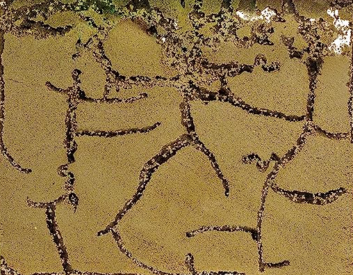
I want to reduce this image to a Boolean map of where the ants have and have not excavated. For a first step, I’ll flatten it to black and white, adjusting brightness and contrast to try to mark the tunnels as black, and the remaining dirt as white. Fortunately, ImageMagick makes this relatively easy:

convert -white-threshold 25% -brightness-contrast 30x100 -alpha off -threshold 50% original.png processed.png

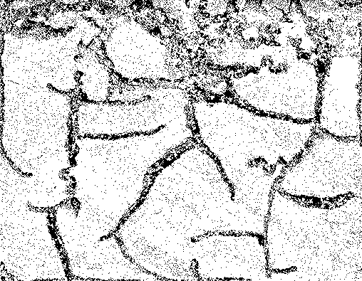
Clearly this is a noisy representation. Some flecks of dirt are dark enough to flatten to ‘black,’ and the ants have left some debris in their tunnels that appear ‘white.’ The background color behind the ant farm is white, so some regions that are particularly well excavated appear bright instead of dark. We might be able to improve that last problem by coloring each pixel according to its distance from either extreme, so that dark tunnels and bright backgrounds are set to ‘black’ and the medium brown dirt is set to ‘white’ - but that’s more involved, and we’ll return to that optimization later if necessary.

In broad strokes, we’ve set excavated space to black and dirt to white. If we aggregate over regions of the image, maybe we can compensate for the noise.

Hexagonal Lattices

My first thought was to overlay a square graph on the image. For each, say, 10x10 pixel region of the image, count the number of black pixels, and if they’re above a cutoff threshold then set the whole square to black, otherwise set it to white. This moves us from a messy image representation to a simpler tile representation, like a board game.

There are a few problems with this approach. Looking ahead, I want to identify rooms and tunnels based on clumps of adjacent black tiles. A square has only four neighbors - eight if we count diagonals, but diagonally-adjacent tiles don’t necessarily imply that the ants have dug a tunnel between the two spaces. So, we’ll use hexagons instead of squares: six-neighbors, no awkwardness about ‘corners,’ and we can still construct a regular lattice:

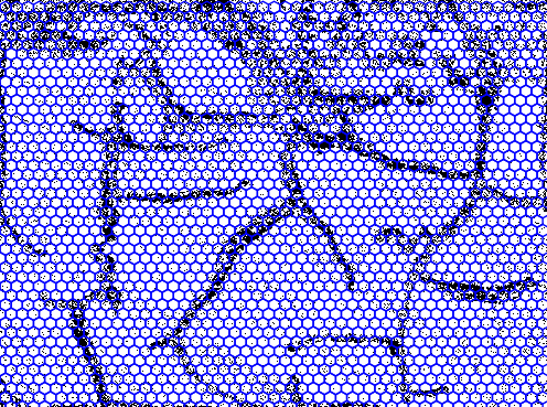
So far so good! A hexagonal coordinate system is a little different from a Cartesian grid, but fortunately I’ve worked with cube coordinates before. For simplicity, we’ll set the diameter of a hexagon to the diameter of a tunnel. This should help us distinguish between tunnels and rooms later on, because tunnels will be around one tile wide, while rooms will be much wider.

Unfortunately, a second problem still remains: there’s no good threshold for how many black pixels should be inside a hexagon before we set it to black. A hexagon smack in the middle of a tunnel should contain mostly black pixels. But what if the hexagons aren’t centered? In a worst-case scenario a tunnel will pass right between two hexagons, leaving them both with half as many black pixels. If we set the threshold too tight then we’ll set both tiles to white and lose a tunnel. If we set the threshold too loose then we’ll set both tiles to black and make a tunnel look twice as wide as is appropriate - perhaps conflating some tunnels with rooms.

So, I’m going to try dithering! This is a type of error propagation used in digital signal processing, typically in situations like converting color images to black and white. In our case, tiles close to white will still be set to white, and tiles close to black will still be darkened to black - but in an ambiguous case where two adjoining tiles are not-quite-dark-enough to be black, we’ll round one tile to white, and the other to black. The result is mostly okay:

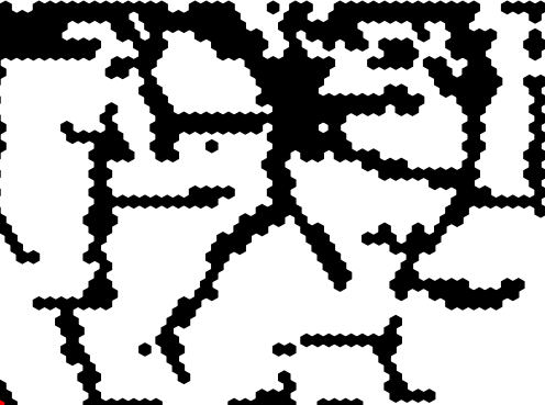
We’re missing some of the regions in the upper right that the ants excavated so completely that the white background shone through. We’re also missing about two hexagons needed to connect the rooms and tunnels on the center-left with the rest of the nest. We might be able to correct both these issues by coloring pixels according to contrast and more carefully calibrating the dithering process, but we’ll circle back to that later.

Flood Filling

So far we’ve reduced a messy color photograph to a much simpler black-and-white tile board, but we still need to identify rooms, junctions, and tunnels. I’m going to approach this with a depth first search:

1. Define a global set of explored tiles, and a local set of “neighborhood” tiles. Select an unexplored tile at random as a starting point.

2. Mark the current tile as explored, add it to the neighborhood, and make a list of unexplored neighbors

3. If the list is longer than three, recursively explore each neighbor starting at step 2

4. Once there are no more neighbors to explore, mark the neighborhood as a “room” if it contains at least ten tiles, and a “junction” if it contains at least four. Otherwise, the neighborhood is part of a tunnel, and should be discarded.

5. If any unexplored tiles remain, select one and go to step 2

Once all tiles have been explored, we have a list of “rooms” and a list of “junctions,” each of which are themselves lists of tiles. We can visualize this by painting the rooms blue and the junctions red:

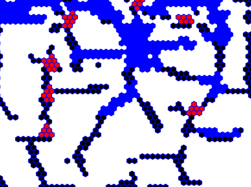
Looking good so far!

Making a Graph

We’re most of the way to a graph representation. We need to create a ‘vertex’ for each room or junction, with a size proportional to the number of tiles in the room, and a position based on the ‘center’ of the tiles.

Then we need to add edges. For this we’ll return to a depth-first flood fill algorithm. This time, however, we’ll recursively explore all tiles adjacent to a room that aren’t part of another room or junction, to see which other vertices are reachable. This won’t preserve the shape, length, or width of a tunnel, but it will identify which areas of the nest are reachable from which others:

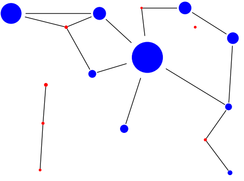
And there we have it!

Drawbacks, Limitations, Next Steps

We’ve gone from a color photo of an ant farm to a network diagram, all using simple algorithms, no fancy machine learning. I think we have a decent result for a clumsy first attempt!

There are many caveats. We’re missing some excavated spaces because of the wall color behind the ant farm in our sample photo. The dithering needs finer calibration to identify some of the smaller tunnels. Most importantly, an enormous number of details need to be calibrated for each ant farm photo. The brightness and contrast adjustments and noise reduction, the hexagon size, the dithering thresholds, and the room and junction sizes for flood filling, may all vary between each colony photo.

For all these reasons, I’m pausing here. If I think of a good way to auto-calibrate those parameters and improve on the image flattening and dithering steps, then maybe I’ll write a part two. Otherwise, this has progressed beyond a couple-evening toy project, so I’ll leave the code as-is.