Predicting Friendships from SMS Metadata

Posted 3/30/2022

We know that metadata is incredibly revealing; given information about who you talk to, we can construct a social graph that shows which social circles you’re in and adjacent to, we can predict your politics, age, and a host of other attributes.

But how does social graph prediction work? How do you filter out noise from “real” social connections? How accurate is it, and in what cases does it make mistakes? This post introduces one approach based on the expectation-maximization algorithm, to start a discussion.

The Setup

We have texting logs from 20 individuals, showing how many times they texted every other participant over the course of a week. We have no additional data, like the timestamps of messages, length, or contents. We also won’t consider the directionality of who sent the texts, just “how many texts were sent between person 1 and 2?” Given these texting logs, we want to find the most probable friendship graph between these 20 people. We will also assume that friendships are always reciprocated, no one-way friends.

We can represent this input as a matrix, where the row and column indicate who is speaking, and the value represents number of texts:

	Person 1	Person 2	Person 3	…
Person 1	0	6	1
Person 2	6	0	11
Person 3	1	11	0
…

It may be tempting to apply a cutoff here. For example, if person 1 and 2 text more than X times we’ll assume they’re friends. However, this doesn’t easily let us represent uncertainty: If the number of texts is close to X, how do we represent how sure we are that they might be friends? Even for values much greater or lower than X, how do we represent our confidence that we haven’t found two non-friends who text a surprising amount, or two friends who text surprisingly infrequently? Instead, we’ll use a slightly more sophisticated approach that lends itself to probability.

We will assume that friends text one another at an unknown rate, and that non-friends text one another at a lower unknown rate. This is a big assumption, and we’ll revisit it later, but for now take it as a given.

We can represent the two texting rates using Poisson distributions. This allows us to ask “what’s the probability of seeing k events (texts), given an underlying rate at which events occur?” The math for this looks like:

We can use this building block to ask a more useful question: Given that we did see k texts, is it more likely that these texts came from a distribution of friends texting, or a distribution of non-friends texting?

This is equivalent to asking “what is the probability that person A and B are friends, given the number of texts sent between them?” So, all we need to do now is run through every pair of people, and calculate the probability that they’re friends!

There’s just one problem: We have no idea what the two texting rates are. To estimate them, we’ll need to add a new level of complexity.

The Model

When determining our friends texting rate and non-friends texting rate, it would be very helpful if we knew the probability that two people are friends. For example, if 80% of all possible friendships exist, then we know most logs of texts represent the logs of friends texting, and only about the lowest 20% of text counts are likely to represent non-friends.

This sounds like it’s making things worse: now we have a third unknown variable, the likelihood of friendship, which we also don’t know the value of! In reality, it will make the problem much easier to solve.

Let’s make a second huge starting assumption: There is an equal likelihood that any two randomly chosen people in the group will be friends. This is generally not true in social graphs - highly charismatic, popular people usually have far more friends, so the probability of friendship is not at all equal - but it will make the math simpler, and it’s not a terrible assumption with only 20 people in our social graph.

We can represent this probability as follows:

To re-iterate the second line, the probability of any given friendship network F is equal to the probability of each friendship in the network existing, times the probability of each non-friendship not existing. In other words, if our friendship probability is 0.8, then about 80% of all possible friendships should exist, and if we propose a friendship network with only five friendships then the above math will tell us that the scenario is highly unlikely.

It’s important to note that this network model represents our prior assumption about the underlying friendship network, but doesn’t lock us in: given enough evidence (text messages) we will override this prior assumption, and add friendship edges even if they are unlikely under a random network.

Next, let’s approach the original problem backwards: Given a friendship network F, what’s the probability that we’d get the text logs we’ve received?

That is, for each friendship that does exist, get the probability of seeing our text observations from the friends texting distribution, and for each friendship that does not exist, get the probability of our text observations from the non-friends texting distribution. Multiply all those probabilities together, and you have the probability of seeing our full set of logs.

The Optimization

We can combine the above pieces and solve in terms of the most likely values for our friends texting rate, our non-friends texting rate, and our friendship probability. I will not include the details in this post, because it’s about five pages of calculus and partial derivatives. The high level idea is that we can take the probability of a friendship network given observed texts and parameters, and take the partial derivative with respect towards one of those parameters. We multiply this across the distribution of all possible friendship networks, weighted by the probability of each network occurring. We set the entire mess equal to zero, and solve for our parameter of interest. When the derivative of a function is zero it’s at either a local minimum or maximum, and for out-of-scope reasons we know that in this context it yields the global maximum. Ultimately, this gives us the most likely value of a parameter, given the probability that each pair of people are friends:

Where n is our number of participants, in this case 20.

But wait! Didn’t the probability that two people are friends depend on the texting rates? How can we solve for the most likely texting rate, based off of the texting rates? We’ll do it recursively:

1. Start with arbitrary guesses as to the values of our two texting rates, and the friendship probability

2. Calculate the probability that each pair of people are friends, based on our three parameters

3. Calculate the most likely values of our three parameters, given the above friendship probabilities

4. Loop between steps 2 and 3 until our three parameters converge

One quick python script to parse the log files and run our four math equations, and:

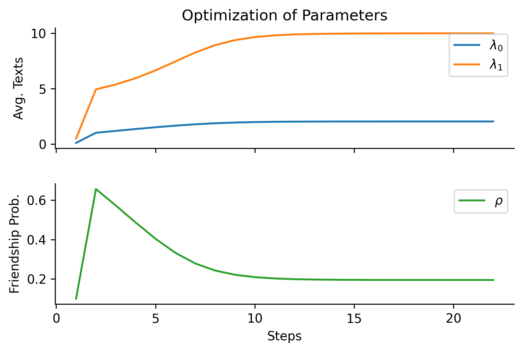
We’ve got an answer! An average of 10 texts per week among friends, 2 among non-friends, and a 20% chance that any two people will be friends. The parameters converge after only 25 steps or so, making this a quick computational optimization.

The Analysis

With our three parameters we can calculate the likelihood that any two individuals are friends based on observed texts, and plot those likelihoods graphically:

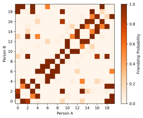
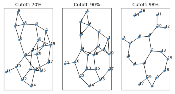
This is our “answer”, but it’s not easy to understand in current form. We’d prefer to render this as a friendship network, where nodes represent people, with an edge between every two people who are friends. How do we translate from this probability matrix to a network? Here, it’s a little more appropriate to apply cutoffs: We can plot all friendships we’re at least 70% confident exist, 90%, and 98%:

Confirmation Test: U.S. Senators

Unconvinced by the “detecting friendships from text messages” example? Let’s apply the exact same code to a similar problem with better defined ground truth: predicting the political party of senators.

We can take data on the voting records for session 1 of the 2021 U.S. Senate. For every pair of senators, we can count the number of times they voted the same way on bills (both voted “yea”, or both voted “nay”). We will assume that senators in the same political party vote the same way at one rate, and senators in different political parties vote together at a lower rate. The signal will be noisy because some senators are absent for some bills, or vote against party lines because of local state politics, occasional flickers of morality, etc.

As in the texting problem, we’ll place an edge between two senators if we believe there is a high chance they are in the same party. We can also anticipate the value of rho: Since the senate is roughly split between Democrats and Republicans, there should be close to a 50% chance that two randomly chosen senators will be in the same party. (This is an even better environment for our “random network” assumption than in the texting friendship network, since all senators will have close to the same degree)

First, the optimization:

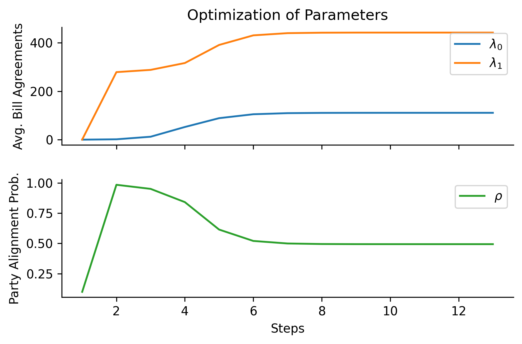
As expected, the probability of any two senators being in the same party is 0.494 - close to 50%. Members of the same party agree on bills roughly 442 times per senate session, while members of opposing parties agree roughly 111 times. And now, the resulting network:

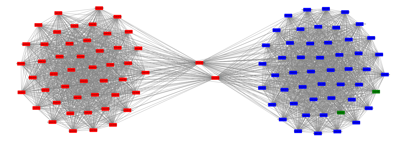
Nodes are colored according to their declared party (red for Republicans, blue for Democrats, green for independents) to confirm the network clusters we’ve found. I’ve also removed the Vice President (who only votes to break ties), and a senator that held a partial term after their predecessor resigned. Since both the Vice President and the short-term senator voted in far fewer bills than their peers, there were no edges between them and other senators.

The remaining results are accurate! Not counting the people I removed because of insufficient voting history, the algorithm struggled to classify two senators, who are shown in the center. These two senators, Collins (R-ME) and Murkowski (R-AK), are considered some of the most moderate Republicans in the senate, and are swing votes. All other senators are clearly placed in the correct cluster with their peers.

Conclusions

We’ve created a model for detecting social relationships from event data. We assume that events occur at a higher rate between people with a social relationship, and a lower rate between people without a relationship. This is general enough to describe a wide variety of scenarios.

But our model also assumes consistency: what if our assumption about two friend texting and non-friend texting rates didn’t hold? For example, in a larger social graph some people may not text much. They still text friends more often than non-friends, but both rates are much lower than their peers. Our current model would mark these less-active users as friendless, and create no edges to them. We could extend our model by switching from two global texting rates to two individual rates, but then we’d have 2N+1 variables to optimize instead of 3, and will need much more training data to optimize.

We also assumed that the underlying social network was a simple random graph: Every two members have an equal chance of being connected to one another. That assumption is appropriate for our senate network, where we’re trying to ascertain group membership. It works relatively well in the texting network because the population is very small. In many scenarios, however, we expect member degree to follow a power law, where a small number of participants are far more connected than others. We could switch our network model from random to many varieties of exponential or scale-free networks, but this will complicate the math and likely add more parameters to tune.

My main takeaway from this is the need to understand assumptions made by the model, which dictate where it can be meaningfully applied, and where it will produce deeply flawed results.