Hex Grids and Cube Coordinates

Posted 2/10/2023

I recently needed to make a graph with a hex lattice shape, like this:

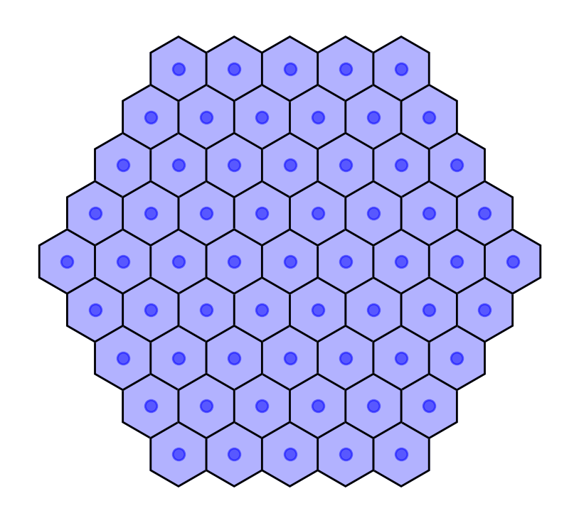
I needed to find distances and paths between different hexagonal tiles, which proved challenging in a cartesian coordinate system. I tried a few solutions, and it was a fun process, so let’s examine each option.

Row and Column (Offset) Coordinates

The most “obvious” way to index hexagonal tiles is to label each according to their row and column, like:

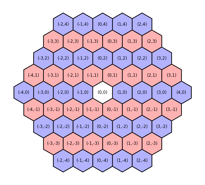
This feels familiar if we’re used to a rectangular grid and cartesian coordinate system. It also allows us to use integer coordinates. However, it has a few severe disadvantages:

1. Moving in the y-axis implies moving in the x-axis. For example, moving from (0,0) to (0,1) sounds like we’re only moving vertically, but additionally shifts us to the right!

2. Coordinates are not mirrored. Northwest of (0,0) is (-1,1), so we might expect that Southeast of (0,0) would be flipped across the vertical and horizontal, yielding (1,-1). But this is not the case! Southeast of (0,0) is (0,-1) instead, because by dropping two rows we’ve implicitly moved twice to the right already (see point one)

These issues make navigation challenging, because the offsets of neighboring tiles depend on the row. Southeast of (0,0) is (0,-1), but Southeast of (0,1) is (1,0), so the same relative direction sometimes requires changing the column, and sometimes does not.

Cartesian Coordinates

Rather than using row and column coordinates we could re-index each tile by its “true” cartesian coordinates:

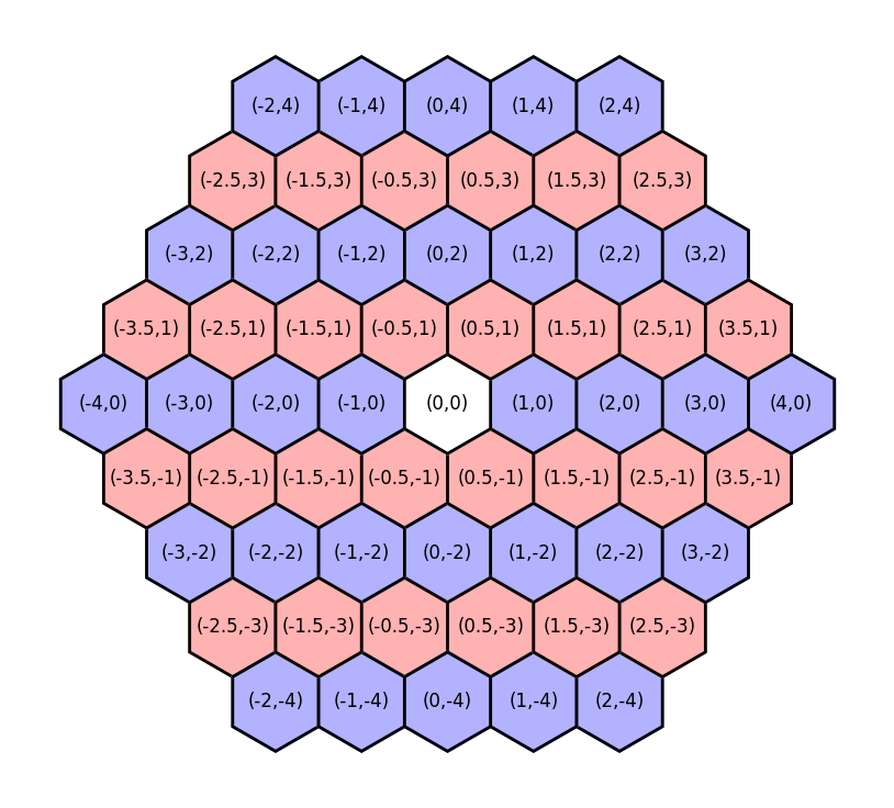
This makes the unintuitive aspects of offset coordinates intuitive:

1. It is now obvious that moving from (0,0) to (0.5,1) implies both a vertical and horizontal change

2. Coordinates now mirror nicely: Northwest of (0,0) is (-0.5,1), and Southeast of (0,0) is (0.5,-1).

3. Following from point 1, it’s now clear why the distance between (0,0) and (3,0) isn’t equal to the distance between (0,0) and (0.5,3).

But while cartesian coordinates are more “intuitive” than offset coordinates, they have a range of downsides:

1. We no longer have integer coordinates. We could compensate by doubling all the coordinates, but then (0,0) is adjacent to (2,0), and keeping a distance of one between adjacent tiles would be ideal.

2. While euclidean-distances are easy to calculate in cartesian space, it’s still difficult to calculate tile-distances using these indices. For example, if we want to find all tiles within two “steps” of (0,0) we need to use a maximum range of about 2.237, or the distance to (1,2).

Cube Coordinates

Fortunately there is a third indexing scheme, with integer coordinates, coordinate mirroring, and easy distance calculations in terms of steps! It just requires thinking in three dimensions!

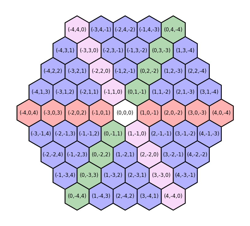
In a cartesian coordinate system we use two axes, since we can move up/down, and left/right. However, on a hexagonal grid, we have three degrees of freedom: we can move West/East, Northwest/Southeast, and Northeast/Southwest. We can define the coordinate of each tile in terms of the distance along each of these three directions, like so:

Why aren’t the cube coordinates simpler?

These “cube coordinates” have one special constraint: the sum of the coordinates is always zero. This allows us to maintain a canonical coordinate for each tile.

To understand why this is necessary, imagine a system where the three coordinates (typically referred to as (q,r,s) to distinguish between systems when we are converting to or from an (x,y) system) correspond directly with the three axes: q refers to distance West/East, r to Northwest/Southeast, and s to Northeast/Southwest. Here’s a visualization of such a scheme:

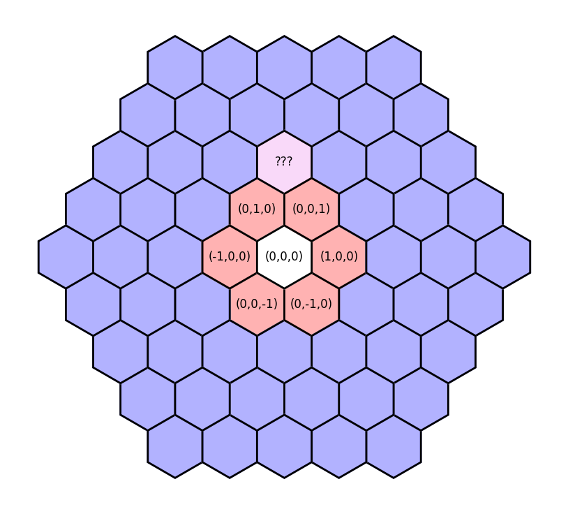
We could take several paths, such as (0,1,1) or (1,2,0) or (-1,0,2), and all get to the same tile! That would be a mess for comparing coordinates, and would make distance calculations almost impossible. With the addition of this “sum to zero” constraint, all paths to the tile yield the same coordinate of (-1,2,-1).

What about distances and coordinate conversion?

Distances in cube coordinates are also easy to calculate - just half the “Manhattan distance” between the two points:

def distance(q1, r1, s1, q2, r2, s2):
        return (abs(q1-q2) + abs(r1-r2) + abs(s1-s2)) / 2

We can add coordinates, multiply coordinates, calculate distances, and everything is simple so long as we remain in cube coordinates.

However, we will unavoidably sometimes need to convert from cube to cartesian coordinates. For example, while I built the above hex grids using cube coordinates, I plotted them in matplotlib, which wants cartesian coordinates to place each hex. Converting to cartesian coordinates will also allow us to find the distance between hex tiles “as the crow flies,” rather than in path-length, which may be desirable. So how do we convert back to xy coordinates?

First, we can disregard the s coordinate. Since all coordinates sum to zero, s = -1 * (q + r), so it represents redundant information, and we can describe the positions of each tile solely using the first two coordinates.

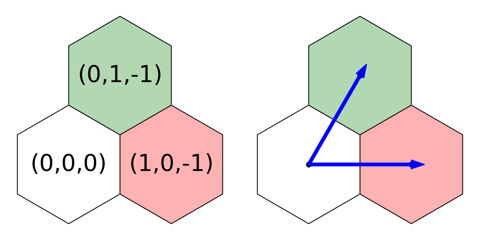
We can also tell through the example above that changing the q coordinate contributes only to changing the x-axis, while changing the r coordinate shifts both the x- and y-axes. Let’s set aside the q coordinate for the moment and focus on how much r contributes to each cartesian dimension.

Let’s visualize the arrow from (0,0,0) to (0,1,-1) as the hypotenuse of a triangle:

We want to break down the vector of length r=1 into x and y components. You may recognize this as a 30-60-90 triangle, or you could use some geometric identities: the internal angles of a hexagon are 120-degrees, and this triangle will bisect one, so theta must be 60-degrees. Regardless of how you get there, we land at our triangle identities:

From here we can easily solve for the x and y components of r, using 2a = r:

We know that (0,1,-1) is halfway between (0,0,0) and (1,0,-1) on the x-axis, so q must contribute twice as much to the x-axis as r does. Therefore, we can solve for the full cartesian coordinates of a hex using the cube coordinates as follows:

This works great! But it leaves the hexagons with a radius of sqrt(3) / 3, which may be inconvenient for some applications. For example, if you were physically manufacturing these hexagons, like making tiles for a board-game, they’d be much easier to cut to size if they had a radius of one. Therefore, you will often see the conversion math from cube to cartesian coordinates written with a constant multiple of sqrt(3), like:

Since this is a constant multiple, it just re-scales the graph, so all the distance measurements and convenient properties of the system remain the same, but hexagons now have an integer radius.

This is the most interesting thing in the world, where do I learn more?

If you are also excited by these coordinate systems, and want to read more about the logic behind cube coordinates, path-finding, line-drawing, wrapping around the borders of a map, and so on, then I highly recommend the Red Blob Games Hexagon article, which goes into much more detail.