Bloom Filters

Posted 4/8/2023

Sticking with a theme from my last post on HyperLogLog I’m writing about more probabilistic data structures! Today: Bloom Filters.

What are they?

Bloom filters track sets: you can add elements to the set, and you can ask “is this element in the set?” and you can estimate the size of the set. That’s it. So what’s the big deal? Most languages have a set in their standard library. You can build them with hash tables or trees pretty easily.

The magic is that Bloom filters can store a set in constant space, while traditional set data structures scale linearly with the elements they contain. You allocate some space when you create the Bloom filter - say, 8 kilobytes of cache space - and the Bloom filter will use exactly 8 kilobytes no matter how many elements you add to it or how large those elements are.

There are two glaring limitations:

1. You cannot enumerate a Bloom filter and ask what elements are in the set, you can only ask whether a specific element may be in the set

2. Bloom filters are probabilistic: they can tell you that an element is not in the set with certainty (no false negatives), but they can only tell you that an element may be in the set, with uncertainty

When creating a Bloom filter, you tune two knobs that adjust their computational complexity and storage requirements, which in turn control their accuracy and the maximum number of unique elements they can track.

Applications

Why would we want a non-deterministic set that can’t tell us definitively what elements it includes? Even if constant-space storage is impressive, what use is a probabilistic set?

Pre-Cache for Web Browsers

Your web-browser stores images, videos, CSS, and other web elements as you browse, so that if you navigate to multiple pages on a website that re-use elements, or you browse from one website to another and back again, it doesn’t need to re-download all those resources. However, spinning hard drives are slow, so checking an on-disk cache for every element of a website will add a significant delay, especially if we learn that we don’t have the element cached and then need to fetch it over the Internet anyway. One solution here is using a Bloom filter as a pre-cache: check whether the URL of a resource is in the Bloom filter, and if we get a “maybe” then we check the disk cache, but if we get a “no” then we definitely don’t have the asset cached and need to make a web request. Because the Bloom filter takes a small and fixed amount of space we can cache it in RAM, even if a webpage contains many thousands of assets.

Pre-Cache for Databases

Databases can use Bloom filters in a similar way. SQL databases are typically stored as binary trees (if indexed well) to faciliate fast lookup times in queries. However, if a table is large, and lots of data must be read from a spinning hard drive, then even a well-structured table can be slow to read through. If queries often return zero rows, then this is an expensive search for no data! We can use Bloom filters as a kind of LOSSY-compressed version of rows or columns in a table. Does a row containing the value the user is asking for exist in the table? If the Bloom filter returns “maybe” then evaluate the query. If the Bloom filter returns “no” then return an empty set immediately, without loading the table at all.

Tracking Novel Content

Social media sites may want to avoid recommending the same posts to users repeatedly in their timeline - but maintaining a list of every tweet that every user has ever seen would require an unreasonable amount of overhead. One possible solution is maintaining a Bloom filter for each user, which would use only a small and fixed amount of space and can identify posts that are definitely new to the user. False positives will lead to skipping some posts, but in an extremely high-volume setting this may be an acceptable tradeoff for guaranteeing novelty.

How do Bloom filters work?

Adding elements

Bloom filters consist of an array of m bits, initially all set to 0, and k hash functions (or a single function with k salts). To add an element to the set, you hash it with each hash function. You use each hash to choose a bucket from 0 to m-1, and set that bucket to 1. In psuedocode:

def add(element)
    for i in 0..k
        bin = hash(element, i) % m
        Bloomfilter[bin] = 1

As a visual example, consider a ten-bit Bloom filter with three hash functions. Here we add two elements:

Querying the Bloom filter

Querying the Bloom filter is similar to adding elements. We hash our element k times, check the corresponding bits of the filter, and if any of the bits are zero then the element does not exist in the set.

def isMaybePresent(element)
    for i in 0..k
        bin = hash(element, i) % m
        if( Bloomfilter[bin] == 0 )
            return false
    return true

For example, if we query ‘salmon’, we find that one of the corresponding bits is set, but the other two are not. Therefore, we are certain that ‘salmon’ has not been added to the Bloom filter:

If all of the corresponding bits are one then the element might exist in the set, or those bits could be the result of a full- or several partial-collisions with the hashes of other elements. For example, here’s the same search for ‘bowfin’:

While ‘bowfin’ hasn’t been added to the Bloom filter, and neither of the added fish have a complete hash collision, the partial hash collisions with ‘swordfish’ and ‘sunfish’ cover the same bits as ‘bowfin’. Therefore, we cannot be certain that ‘bowfin’ has or has not been added to the filter.

Estimating the Set Length

There are two ways to estimate the number of elements in the set. One is to maintain a counter: every time we add a new element to the set, if those bits were not all already set, then we’ve definitely added a new item. If all the bits were set, then we can’t distinguish between adding a duplicate element and an element with hash collisions.

Alternatively, we can retroactively estimate the number of elements based on the density of 1-bits, the number of total bits, and the number of hash functions used, as follows:

In other words, the density of 1-bits should correlate with the number of elements added, where we add k or less (in the case of collision) bits with each element.

Both estimates will begin to undercount the number of elements as the Bloom filter “fills.” Once many bits are set to one, hash collisions will be increasingly common, and adding more elements will have little to no effect on the number of one-bits in the filter.

Configurability

Increasing the number of hash functions lowers the chance of a complete collision. For example, switching from two hash functions to four means you need twice as many bits to be incidentally set by other elements of the set before a query returns a false positive. While I won’t include the full derivation, the optimal number of hash functions is mathematically determined by the desired false-positive collision rate (one in a hundred, one in a thousand, etc):

However, increasing the number of hash functions also fills the bits of the Bloom filter more quickly, decreasing the total number of elements that can be stored. We can compensate by storing more bits in the Bloom filter, but this increases memory usage. Therefore, the optimal number of bits in a Bloom filter will also be based on the false-positive rate, and on the number of unique elements we expect to store, which will determine how “full” the filter bits will be.

If we want to store more elements without increasing the error rate, then we need more bits to avoid further collisions. If we want to insert the same number of elements and a lower error-rate, then we need more bits to lower the number of collisions. If we deviate from this math by using too few bits or too many hash functions then we’ll quickly fill the filter and our error rate will skyrocket. If we use fewer hash functions then we’ll increase the error-rate through sensitivity to collisions, unless we also increase the number of bits, which can lower the error-rate at the cost of using more memory than necessary.

Note that this math isn’t quite right - we need an integer number of hash functions, and an integer number of bits, so we’ll round both to land close to the optimal configuration.

How well does this work in practice?

Let’s double-check the theoretical math with some simulations. I’ve inserted between one and five-thousand elements, and used the above equations to solve for optimal Bloom filter parameters for a desired error rate of 1%, 5%, and 10%.

Here’s the observed error rate, and the number of recommended hash functions, plotted using the mean result and a 95% confidence-interal:

As we can see, our results are almost spot-on, and become more reliable as the Bloom filter increases in size! Here are the same simulation results, where the hue represents the number of bits used rather than the number of hash functions:

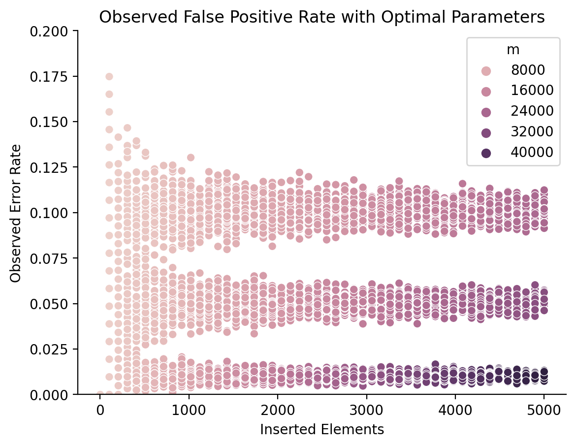
Since the number of recommended bits changes with the number of inserted elements, I had to plot this as a scatter plot rather than a line plot. We can see that the number of bits needed steadily increases with the number of inserted elements, but especially with the error rate. While storing 5000 elements with a 5% error rate requires around 24-kilobits, maintaining a 1% error rate requires over 40 kilobits (5 kilobytes).

Put shortly, the math checks out.

Closing Thoughts

I think I’m drawn to these probabilistic data structures because they loosen a constraint that I didn’t realize existed to do the “impossible.”

Computer scientists often discuss a trade-off between time and space. Some algorithms and data structures use a large workspace to speed computation, while others can fit in a small amount of space at the expense of more computation.

For example, inserting elements into a sorted array runs in O(n) - it’s quick to find the right spot for the new element, but it takes a long time to scoot all the other elements over to make room. By contrast, a hash table can insert new elements in (amortized) O(1), meaning its performance scales much better. However, the array uses exactly as much memory as necessary to fit all its constituent elements, while the hash table must use several more times memory - and keep most of it empty - to avoid hash collisions. Similarly, compression algorithms pack data into more compact formats, but require additional computation to get useful results back out.

However, if we loosen accuracy and determinism, creating data structures like Bloom filters that can only answer set membership with a known degree of confidence, or algorithms like Hyperloglog that can count elements with some error, then we can create solutions that are both time and space efficient. Not just space efficient, but preposterously so: constant-space solutions to set membership and size seem fundamentally impossible. This trade-off in accuracy challenges my preconceptions about what kind of computation is possible, and that’s mind-blowingly cool.