
Bayesian Network Science
Posted 1/26/2026
I am currently teaching masters students to perform statistical network analysis, especially predicting the structure of a network from observational data, calibrating network models to real-world data, and rejecting hypotheses about the structure of networks. This post repurposes my recent lecture for a more general audience. It is more math-heavy than most of my posts, and involves some statistics and light differential equations, and assumes some familiarity with graph theory or network science.
What is Bayesian Statistics?
Statistical techniques can be broadly put in two categories:
-
Frequentist Statistics uses evidence to estimate a point value. Probabilities are interpreted as long run frequencies.
-
Bayesian Statistics uses evidence and a set of prior beliefs to produce a posterior distribution of potential point values. Probabilities are interpreted as subjective degrees of belief.
For a crude example, say we flip a coin many times. In frequentist statistics we say that the probability of heads is the fraction of heads over the number of flips, so if P(heads) = 0.5 then over many coin flips about half of the flips should come out heads.
In Bayesian statistics we have a prior belief about the fairness of the coin, expressed as a distribution. A normal distribution centered at 0.5 means “I believe the coin is fair, but I wouldn’t be so surprised if it was a tiny bit biased towards heads or tails. As the bias increases, so does my surprise.”
By contrast, a uniform prior would indicate “I have no idea whether the coin is biased, I would believe all biases equally.” A uniform prior makes Bayesian statistics behave like frequentist statistics: our result will be based solely on the coin flips we observe.
As we flip the coin we gather evidence, and update our posterior distribution, indicating our current belief about the coin’s nature. The posterior distribution functions much like the prior distribution: “based on our priors and gathered evidence, we would be most confident that the coin’s bias is 0.49, but 0.48 and 0.50 wouldn’t be so surprising, and 0.8 would be much more surprising.”
Given enough evidence, Bayesian and frequentist statistics will converge to the same answer. If we flip the coin a million times and it clearly turns heads 80% of the time then any Bayesian will yield, “my priors were wrong, the evidence is overwhelming.” However, given limited evidence and an accurate prior, Bayesian techniques can converge more quickly. The Bayesian style of thinking is well-suited to network inference tasks, where we have a model, some prior beliefs about the parameters of that model, and gathered evidence about a network.
Bayes’ Theorem
A foundation of Bayesian statistics is Bayes’ theorem (Bae’s theorem if you really love Bayesian stats) which allows us to take a formula for the probability of observations given a model configuration, and invert it to obtain the probability of a model configuration given our observations. The theorem is as follows:
Or, in Bayesian language:
I find this equation impenetrably dense without an example. Say we’re in a windowless room and a student walks in with wet hair, and I want to know whether it’s raining. I can say:
That is, the probability that it’s raining given that someone walked in with wet hair is based on:
- The probability that they’d have wet hair if it were raining. Are they carrying an umbrella?
- The probability that it’s raining. If we are in a desert then there are likely better explanations.
- The probability that the student’s hair is wet. If their hair is always wet (maybe they take a shower right before office hours) then this is not a useful signal.
Bayesian Statistics in Network Science
We use Bayesian statistics in two ways during network analysis:
- Predicting model parameters given a network generated by the model
- Predicting edges based on observations, given an underlying model
Estimating p from a G(n,p) graph
Say we have an adjacency matrix A. That is, a 2D matrix of zeros and ones such that A[i,j] indicates whether there is an edge from node i to j (if A[i,j]=1), or not (A[i,j]=0). This is an undirected graph, so A[i,j]=A[j,i]. We think this matrix was generated by an Erdős-Rényi random graph: that is, every possible edge exists with a uniform probability p. We want to estimate that p value. We’ll start with the opposite problem: given an ER graph parameterized by p, what is the probability of generating adjacency matrix A?
How many edges should we expect in an ER graph with n nodes and p edge probability? Well, we know there are N(N-1)/2 possible edges (every node can connect to every node except itself, divide by 2 because a->b and b->a represent the same edge), or N choose 2, and each occurs with probability p, so for m edges we can expect m = p * (N choose 2). But let’s work from the opposite direction. If each edge exists with probability p, then the probability of generating a given graph is:
That is, every edge that exists in the graph should exist with probability p, and every edge that does not exist in the graph will be absent with probability 1 - p. We can rewrite the expression more concisely:
For convenience, let’s reparameterize in terms of the size of the graph with m edges and n vertices:
That is, the likelihood of generating a graph is given by the probability of an edge for each edge that exists (m), times the probability of no edge for each edge does not exist (n choose 2 possible edges, minus the m edges that actually exist).
Now, given a graph A, what is the most likely p? We want argmax p of l(p), or the p that maximizes the likelihood of the graph. How do we solve for this? With partial derivatives and maximum likelihood estimation (MLE). Specifically, we want to set the partial derivative of l(p) with respect to p to zero:
When the derivative is zero we have an inflection point, typically a local maxima, minima, or saddle point. However, because the likelihood is a concave function we know there will only be one inflection point at the global maxima.
Useful fact: The argmax of l(p) will also be the argmax of log l(p). Why useful? Because in logs products become sums, which are much easier to differentiate. Additionally, our probabilities will often be very tiny, which presents numeric instability with floating point numbers. Logarithms will boost our probabilities into a higher range and stabilize calculations.
This matches our intuition: the edge probability is equal to the graph density, which is the percentage of possible edges that actually exist. Success!
Toy Example
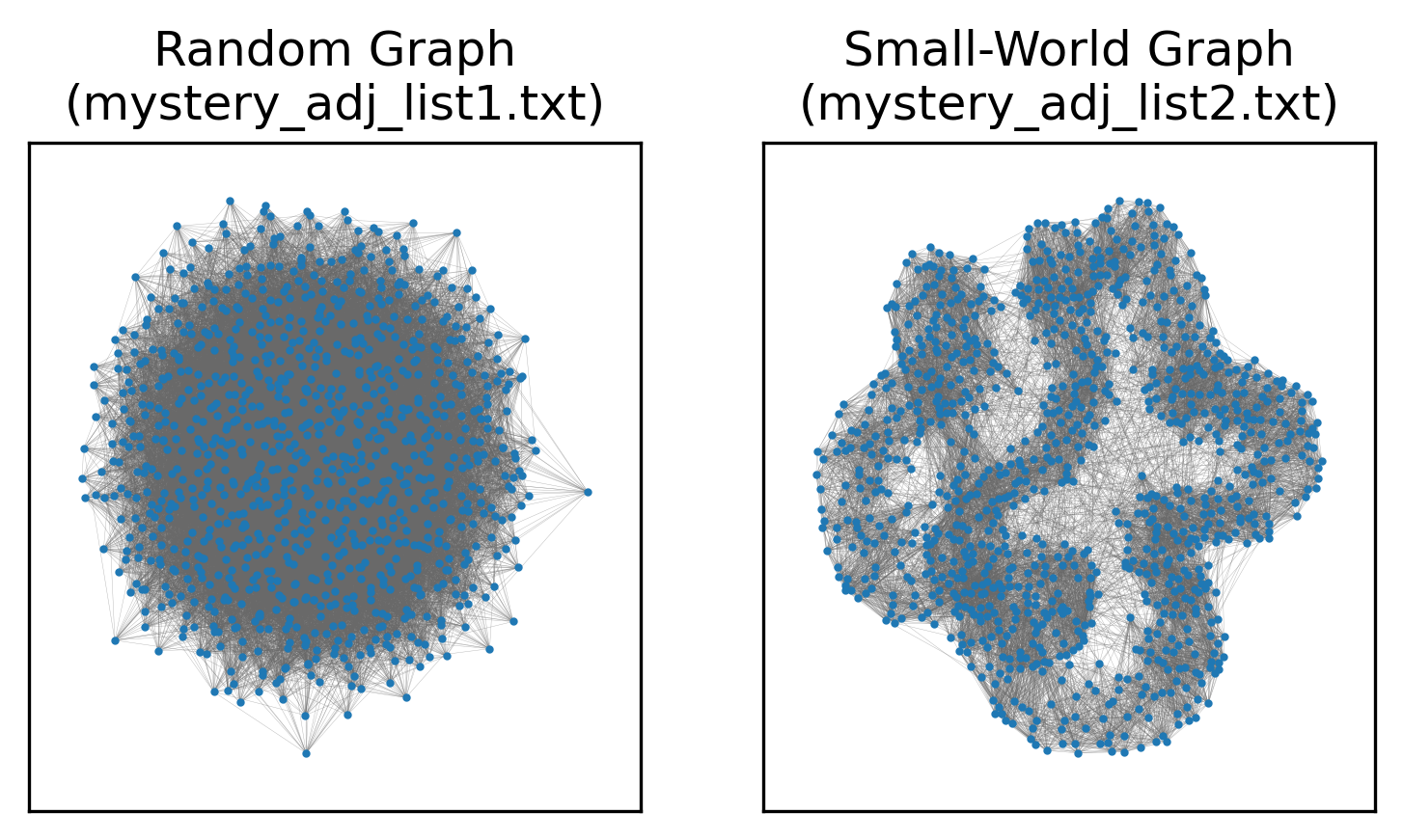
I’ve prepared two networks which you can find here. We want to know whether they are random graphs or not. To determine this, let’s fit a G(n,p) random graph model to each dataset.
1
2
3
4
5
6
7
8
9
10
11
12
13
14
15
16
#!/usr/bin/env python3
import networkx as nx
import pandas as pd
import seaborn as sns
import matplotlib.pyplot as plt
import math

def estimateP(G):
    edges = G.number_of_edges()
    return edges / math.comb(G.number_of_nodes(), 2)

G1 = nx.read_adjlist("data/mystery_adj_list1.txt")
G2 = nx.read_adjlist("data/mystery_adj_list2.txt")

p1 = estimateP(G1)
p2 = estimateP(G2)
Now we will produce a hundred random graphs with those parameters, measure some attributes of those networks, and compare our two real networks to the reference distributions. If our real graphs are random, they should fall comfortably within the bell curve of similar networks. If they are not random, some attributes may fall well outside the reference distributions.
1
2
3
4
5
6
7
8
9
10
11
12
13
14
15
16
17
18
19
20
21
22
23
24
25
26
27
28
29
30
31
32
33
def generateNetworks(n, p, c):
    networks = []
    for i in range(c):
        G = nx.gnp_random_graph(n,p)
        networks.append(G)
    return networks

ref1 = generateNetworks(G1.number_of_nodes(), p1, 100)
ref2 = generateNetworks(G2.number_of_nodes(), p2, 100)

rows = []
for G in ref1:
    t = nx.transitivity(G)
    a = nx.average_shortest_path_length(G)
    d = nx.degree_assortativity_coefficient(G)
    rows.append((t,a,d,"1"))
for G in ref2:
    t = nx.transitivity(G)
    a = nx.average_shortest_path_length(G)
    d = nx.degree_assortativity_coefficient(G)
    rows.append((t,a,d,"2"))
df = pd.DataFrame(rows, columns=["Transitivity", "Avg. Shortest Path Length", "Assortativity", "Distribution"])

df2 = df.melt(id_vars=["Distribution"], var_name="Metric")
g = sns.FacetGrid(df2, col="Metric", row="Distribution", sharex=False, sharey=False, despine=False, margin_titles=True)
g.map(sns.kdeplot, "value")
g.axes[0,0].axvline(x=nx.transitivity(G1), color='r')
g.axes[0,1].axvline(x=nx.average_shortest_path_length(G1), color='r')
g.axes[0,2].axvline(x=nx.degree_assortativity_coefficient(G1), color='r')
g.axes[1,0].axvline(x=nx.transitivity(G2), color='r')
g.axes[1,1].axvline(x=nx.average_shortest_path_length(G2), color='r')
g.axes[1,2].axvline(x=nx.degree_assortativity_coefficient(G2), color='r')
plt.show()
As we can see, the top row, representing the first network and reference distributions, looks plausibly random. The graph’s transitivity, average shortest path length, and degree assortativity are all well-within range for ER networks with the same number of nodes and edges. By contrast, the bottom row is clearly not random: the degree assortativity is similar to that of a random network, but transitivity and shortest path length are definitively not. In fact, the second network comes from the Watts-Strogatz small-world model. Similar number of nodes and edges, similar degree sequence, very different structure.
A visual comparison of the networks would also make the difference clear, but we’re working with statistics today, not guessing at network models from images:
These tools are sufficient to take a mathematical model for network generation, calibrate it to real-world data to find the parameters most likely to yield the observed network, and then used the tuned model to determine whether the network was plausibly generated by such a model. This can help us categorize networks and definitely say “this network is not random,” “this network may have a powerlaw degree sequence, but has structure that is decidedly not explained by the preferential attachment of the Barabasi-Albert model,” and so on.
In the next post, we will explore inferring what edges in a network might exist by applying statistical analysis to observations of interactions.