Image Dithering in Color!

Posted 1/17/2023

In my last post I demonstrated how to perform image dithering to convert colored images to black and white. This consists of converting each pixel to either black or white (whichever is closer), recording the amount of “error,” or the difference between the original luminoscity and the new black/white value, and propagating this error to adjoining pixels to brighten or darken them in compensation. This introduces local error (some pixels will be converted to white when their original value is closer to black, and vice versa), but globally lowers error, producing an image that appears much closer to the original.

I’m still playing with dithering, so in this post I will extend the idea to color images. Reducing the number of colors in an image used to be a common task: while digital cameras may be able to record photos with millions of unique colors, computers throughout the 90s often ran in “256 color” mode, where they could only display a small range of colors at once. This reduces the memory footprint of images significantly, since you only need 8-bits per pixel rather than 24 to represent their color. Some image compression algorithms still use palette compression today, announcing a palette of colors for a region of the image, then listing an 8- or 16-bit palette index for each pixel in the region rather than a full 24-bit color value.

Reducing a full color image to a limited palette presents a similar challenge to black-and-white image dithering: how do we choose what palette color to use for each pixel, and how do we avoid harsh color banding?

We’ll start with a photo of a hiking trail featuring a range of greens, browns, and whites:

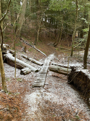
Let’s reduce this to a harsh palette of 32 colors. First, we need to generate such a palette:

#!/usr/bin/env python3
import numpy as np

def getPalette(palette_size=32):
    colors = []
    values = np.linspace(0, 0xFFFFFF, palette_size, dtype=int)
    for val in values:
        r = val >> 16
        g = (val & 0x00FF00) >> 8
        b = val & 0x0000FF
        colors.append((r,g,b))
    return colors

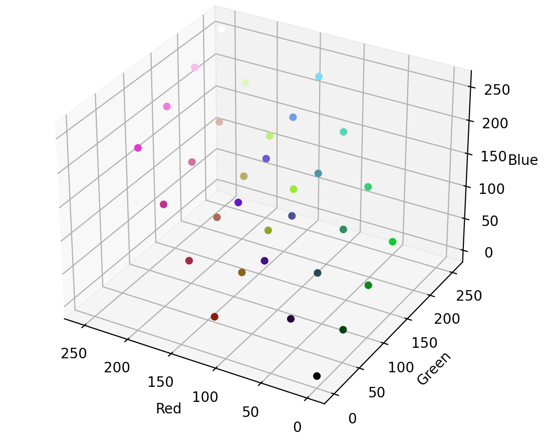
I don’t know much color theory, so this is far from an “ideal” spread of colors. However, it is 32 equally spaced values on the numeric range 0x000000 to 0xFFFFFF, which we can convert to RGB values. We can think of color as a three dimensional space, where the X, Y, and Z axes represent red, green, and blue. This lets us visualize our color palette as follows:

import matplotlib.pyplot as plt

def plotPalette(palette):
    fig = plt.figure(figsize=(6,6))
    ax = fig.add_subplot(111, projection='3d')
    r = []
    g = []
    b = []
    c = []
    for color in palette:
        r.append(color[0])
        g.append(color[1])
        b.append(color[2])
        c.append("#%02x%02x%02x" % color)
    g = ax.scatter(r, g, b, c=c, marker='o', depthshade=False)
    ax.invert_xaxis()
    ax.set_xlabel('Red')
    ax.set_ylabel('Green')
    ax.set_zlabel('Blue')
    plt.show()

Which looks something like:

Just as in black-and-white image conversion, we can take each pixel and round it to the closest available color - but instead of two colors in our palette, we now have 32. Here’s a simple (and highly inefficient) conversion:

# Returns the closest rgb value on the palette, as (red,green,blue)
def getClosest(color, palette):
    (r,g,b) = color
    closest = None #(color, distance)
    for p in palette:
        # A real distance should be sqrt(x^2 + y^2 + z^2), but
        # we only care about relative distance, so faster to leave it off
        distance = (r-p[0])**2 + (g-p[1])**2 + (b-p[2])**2
        if( closest == None or distance < closest[1] ):
            closest = (p,distance)
    return closest[0]

def reduceNoDither(img, palette, filename):
    pixels = np.array(img)
    for y,row in enumerate(pixels):
        for x,col in enumerate(row):
            pixels[y,x] = getClosest(pixels[y,x], palette)
    reduced = Image.fromarray(pixels)
    reduced.save(filename)

img = Image.open("bridge.png")
palette = getPalette()
reduceNoDither(img, palette, "bridge_32.png")

The results are predictably messy:

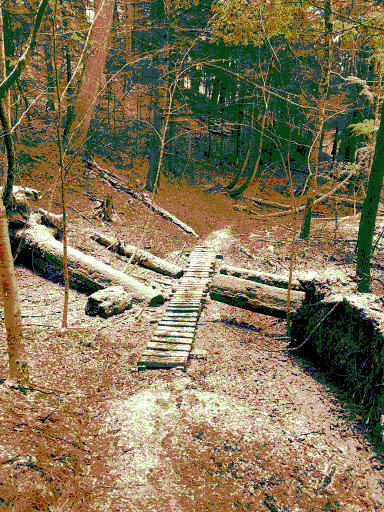
Our palette only contains four colors close to brown, and most are far too red. If we convert each pixel to the closest color on the palette, we massively over-emphasize red, drowning out our greens and yellows.

Dithering to the rescue! Where before we had an integer error for each pixel (representing how much we’d over or under-brightened the pixel when we rounded it to black/white), we now have an error vector, representing how much we’ve over or under emphasized red, green, and blue in our rounding.

As before, we can apply Atkinson dithering, with the twist of applying a vector error to three dimensional color points:

# Returns an error vector (delta red, delta green, delta blue)
def getError(oldcolor, newcolor):
    dr = oldcolor[0] - newcolor[0]
    dg = oldcolor[1] - newcolor[1]
    db = oldcolor[2] - newcolor[2]
    return (dr, dg, db)

def applyError(pixels, y, x, error, factor):
    if( y >= pixels.shape[0] or x >= pixels.shape[1] ):
        return # Don't run off edge of image
    er = error[0] * factor
    eg = error[1] * factor
    eb = error[2] * factor
    pixels[y,x,RED] += er
    pixels[y,x,GREEN] += eg
    pixels[y,x,BLUE] += eb

def ditherAtkinson(img, palette, filename):
    pixels = np.array(img)
    total_pixels = pixels.shape[0] * pixels.shape[1]
    for y,row in enumerate(pixels):
        for x,col in enumerate(row):
            old = pixels[y,x] # Returns reference
            new = getClosest(old, palette)
            quant_error = getError(old, new)
            pixels[y,x] = new
            applyError(pixels, y,   x+1, quant_error, 1/8)
            applyError(pixels, y,   x+2, quant_error, 1/8)
            applyError(pixels, y+1, x+1, quant_error, 1/8)
            applyError(pixels, y+1, x,   quant_error, 1/8)
            applyError(pixels, y+1, x-1, quant_error, 1/8)
            applyError(pixels, y+2, x,   quant_error, 1/8)
    dithered = Image.fromarray(pixels)
    dithered.save(filename)

Aaaaaand presto!

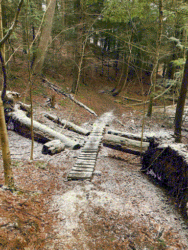
It’s far from perfect, but our dithered black and white images were facsimiles of their greyscale counterparts, too. Pretty good for only 32 colors! The image no longer appears too red, and the green pine needles stand out better. Interestingly, the dithered image now appears flecked with blue, with a blue glow in the shadows. This is especially striking on my old Linux laptop, but is more subtle on a newer screen with a better color profile, so your mileage may vary.

We might expect the image to be slightly blue-tinged, both because reducing red values will make green and blue stand out, and because we are using an extremely limited color palette. However, the human eye is also better at picking up some colors than others, so perhaps these blue changes stand out disproportionately. We can try compensating, by reducing blue error to one third:

That’s an arbitrary and unscientific compensation factor, but it’s removed the blue tint from the shadows in the image, and reduced the number of blue “snow” effects, suggesting there’s some merit to per-channel tuning. Here’s a side-by-side comparison of the original, palette reduction, and each dithering approach:

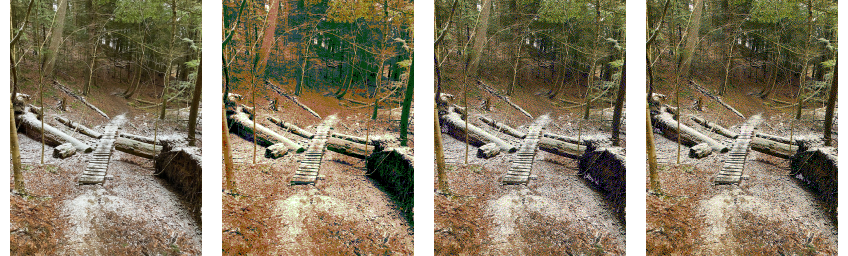
Especially at a smaller resolution, we can do a pretty good approximation with a color selection no wider than a big box of crayons. Cool!