
Word Prominence: A Primer
Posted 6/9/2025
A common task in natural language processing is determining what a text (a book, speech, tweet, email) is about. At its simplest, we may start by asking what words appear most prominently in a text, in the hope that they’ll be topic key-words. Here “prominence” is when a word appears disproportionately in this text compared to others. For example, “the,” “a,” and “and” will always appear with high frequency, but they appear with high frequency in every text and are uninteresting to us.
Our approach will start by reducing a text to a list of words and a count of how many times they occur, typically referred to as a bag of words model. This destroys sentence structure and context, a little like burning an essay and sifting through the ashes, but hey, it keeps the math simple, and you have to start somewhere.
For all of the techniques outlined below we’ll need two texts: the text we’re interested in studying, and a “baseline” corpus of text for comparison.
TF-IDF
Our first contender for identifying keywords is term-frequency inverse-document-frequency or TF-IDF. For each word in our text of interest we’ll first measure the frequency with which it occurs, or literally the number of times the word appears divided by the total number of words in the text. For example in Python, if t is a particular term and d is a dictionary of words and how many times they appear, then:
1
2
3
def tf(t, d):
    total = sum(d.values())
    return d[t] / total
Then we’ll examine a number of other texts for comparison, and count how many of those texts contain the target word. Formally the inverse document frequency is defined as:
Or in Python, if D is a list of documents (where each document is a dictionary of terms and how many times they appear, as in tf):
1
2
3
4
5
6
def idf(t, D):
    total = 0
    for d in D:
        if( t in d.keys() ):
            total += 1
    return math.log(len(D) / total)
This means if a term appears in all N documents we’ll get idf(t, D) = log(N/N) = 0, and the fewer documents a term appears in, the higher its IDF score will be.
We can combine term-frequency and inverse-document frequency as simply term-frequency times inverse document frequency, or:
Now terms that appear in many documents will get a low score, and terms that appear in the target document with low frequency will get a low score, but terms that appear with relatively high frequency in the text of interest and appear in few other documents will get a high score.
What does this get us in practice? Well, to borrow Wikipedia’s example, we can compare every play by Shakespeare (I grabbed the Comedy, History, and Tragedy selection from here). Here are the top terms in Romeo and Juliet, sorted by their TF-IDF scores:
| Word | TF | IDF | TF-IDF |
|---|---|---|---|
| romeo | 0.0097 | 3.6109 | 0.0350 |
| juliet | 0.0057 | 2.9178 | 0.0166 |
| capulet | 0.0045 | 3.6109 | 0.0164 |
| mercutio | 0.0028 | 3.6109 | 0.0100 |
| benvolio | 0.0025 | 3.6109 | 0.0091 |
| tybalt | 0.0024 | 3.6109 | 0.0086 |
| laurence | 0.0024 | 2.9178 | 0.0070 |
| friar | 0.0031 | 1.5315 | 0.0047 |
| montague | 0.0013 | 2.9178 | 0.0039 |
| paris | 0.0018 | 1.4137 | 0.0026 |
| nurse | 0.0046 | 0.5664 | 0.0026 |
| sampson | 0.0007 | 2.9178 | 0.0019 |
| balthasar | 0.0006 | 2.5123 | 0.0014 |
| gregory | 0.0006 | 2.0015 | 0.0012 |
| peter | 0.0009 | 1.3083 | 0.0012 |
| mantua | 0.0004 | 2.5123 | 0.0011 |
| thursday | 0.0004 | 2.5123 | 0.0011 |
The top terms in the play by term frequency are “and,” “the,” and “I,” which each appear about 2% of the time - but these terms all have IDF scores of zero because they appear in every play, and so receive a TF-IDF score of zero as well.
However, only one play includes “Romeo.” This makes up almost 1% of Romeo and Juliet - very common, the twelfth most common or so word - but top of the list by TF-IDF standards.
TF-IDF isn’t perfect - it’s identified many of the names of characters, but also words like “Thursday” and “Paris” (not the setting, which is Verona, Italy) that aren’t especially central to the plot. Nevertheless, TF-IDF is impressively effective given its simplicity. So where does it really fall flat?
The biggest shortcoming of IDF is that it’s boolean: a term either appears in a document or not. However, in large corpora of text we often require more nuance than this. Consider trying to identify what topics a subreddit discusses by comparing comments in the subreddit to comments in other subreddits. In 2020 people in practically every subreddit were discussing COVID-19 - it impacted music festivals, the availability of car parts, the cancellation of sports games, and had some repercussion in almost every aspect of life. In this setting Covid would have an IDF score of near zero, but we may still want to identify subreddits that talk about Covid disproportionately to other communities.
Jensen-Shannon Divergence
Jensen-Shannon Divergence, or JSD, compares term frequencies across text corpora directly rather than with an intermediate “does this word appear in a document or not” step. At first this appears trivial: just try tf(t, d1) - tf(t, d2) or maybe tf(t, d1) / tf(t, d2) to measure how much a term’s frequency has changed between documents 1 and 2.
The difference between term frequencies is called a proportion shift, and is sometimes used. Unfortunately, it has a tendency to highlight uninteresting words. For example, if “the” occurs 2% of the time in one text and 1.5% of the time in another text, that’s a shift of 0.5%, more than Capulet’s 0.45%.
The second approach, a ratio of term frequencies, is more appealing. A relative change in frequencies may help bury uninteresting “stop words” like “the,” “a,” and “it,” and emphasize more significant shifts. However, there’s one immediate limitation: if a term isn’t defined in d2 then we’ll get a division-by-zero error. Some frequency comparisons simply skip over words that aren’t defined in both corpora, but these may be the exact topic words that we’re interested in. Other frequency comparisons fudge the numbers a little, adding 1 to the number of occurrences of every word to ensure every term is defined in both texts, but this leads to less mathematical precision, especially when the texts are small.
Jensen-Shannon Divergence instead compares the frequency of words in one text corpus against the frequency of words in a mixture corpus M:
Here, M is defined as the average frequency with which a term appears in the two texts, or M=1/2 * (P+Q). This guarantees that every term from texts P and Q will appear in M. Additionally, D refers to the Kullback-Leibler Divergence, which is defined as:
The ratio of frequencies gives us a measure of how much the term prominence has shifted, and multiplying by P(x) normalizes our results. In other words, if the word “splendiforous” appears once in one book and not at all in another then that might be a large frequency shift, but P(x) is vanishingly small and so we likely don’t care.
Note that JSD is defined in terms of the total amount that two texts diverge from one another. In this case we’re interested in identifying the most divergent terms between two texts rather than the total divergence, so we can simply rank terms by P(x) * log(P(x)/M(x)). Returning to our Romeo and Juliet example, such a ranking comparing the play to Othello (made by the Shifterator package) might look like:
Jensen-Shannon Divergence can find prominent terms that TF-IDF misses, and doesn’t have any awkward corners with terms that only appear in one text. However, it does have some limitations:
-
First, JSD is sensitive to text size imbalance: the longer a text is, the smaller a percentage each word in the text is likely to appear with, so measuring change in word prominence between a small and large text will indicate that all the words in the short text have higher prominence. To some extent this problem is fundamental - you can’t meaningfully compare word prominence between a haiku and a thousand-page book - but some metrics are more sensitive to size imbalances than others.
-
Second, KLD has a built-in assumption: frequency shifts for common words are more important than frequency shifts for uncommon words. For example, if a word leaps in frequency from 0.00005 to 0.00010 then its prominence has doubled, but it remains an obscure word in both texts. Multiplying the ratio of frequencies by
P(x)ensures that only words that appear an appreciable amount will have high divergence. What’s missing is a tuning parameter: how much should we prefer shifts in common terms to shifts in uncommon terms? Should there be a linear relationship between frequency and how much we value a frequency shift, or should it be an exponential relationship?
These two shortcomings led to the development of the last metric I’ll discuss today.
Rank-Turbulence Divergence
Rank-Turbulence Divergence is a comparatively new metric by friends at the Vermont Complex Systems Institute. Rather than comparing term frequency it compares term rank. That is, if a term moves from the first most prominent (rank 1) to the fourth (rank 4) that’s a rank shift of three. In text, term frequency tends to follow a Zipf distribution such that the rank 2 term appears half as often as the rank 1 term, and the rank 3 term a third as much as rank 1, and so on. Therefore, we can measure the rank as a proxy for examining term frequency. This is convenient, because rank does not suffer from the “frequency of individual terms decreases the longer the text is” challenge that JSD faces.
Critically, we do need to discount changes in high rank (low frequency) terms. If a term moves from 2nd most prominent to 12th most prominent, that’s a big change. If a term moves from 1508th most prominent to 1591st, that’s a little less interesting. However, instead of multiplying by the term frequency as in KLD, Rank Turbulence Divergence offers an explicit tuning parameter for setting how much more important changes in low rank terms are than high rank.
For words that appear in one text but not another, rank turbulence divergence assigns them the highest rank in the text. For example, if text 1 contains 200 words, but not “blueberry,” then blueberry will have rank 201, as will every other word not contained in the text. This is principled, because we aren’t assigning a numeric value to how often the term appears, only truthfully reporting that words like “blueberry” appear less than every other term in the text.
The math at first looks a little intimidating:
Even worse, that “normalization factor” is quite involved on its own:
However, the heart of the metric is in the absolute value summation:
If all we want to do is identify the most divergent terms in each text, and not measure the overall divergence of the two systems, then this snippet is enough. It also builds our intuition for the metric: all we’re really doing is measuring a change in inverse rank, with a knob to tune how much we emphasize changes for common words. The knob ranges from 0 (high and low ranked terms are equally “important”) to infinity (massively emphasize shifts in common words, ignoring shifts in rare words). Here’s an example plotting the difference in words used on two subreddits, r/NoNewNormal (which was a covid conspiracy group) and r/CovIdiots (which called out people acting foolishly during the pandemic):
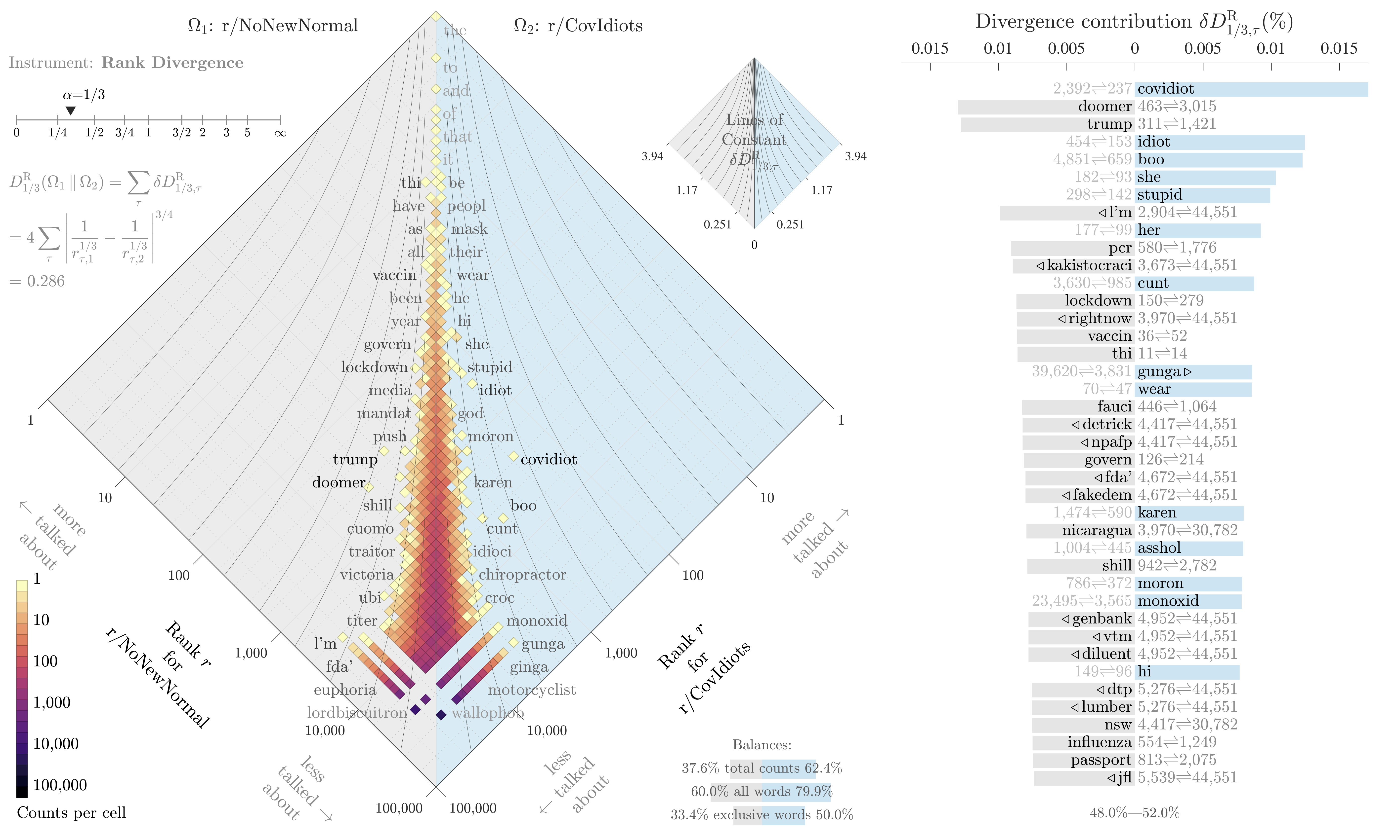
The “divergence contribution” plot on the right can be read like Shifterator’s JSD plot, and simply lists the most divergent terms and which text they appear more in. The allotaxonometry plot on the left reads like a scatterplot, where one axis is the rank of words in r/NoNewNormal and the other axis is the rank of words in r/CovIdiots. When words have the same rank in both texts they’ll appear on the center line, and the more they skew towards one subreddit or another the further out they’ll be plotted. Only a small subset of notable words are explicitly labeled, and the rest of the plot operates more like a heatmap to give a sense of how divergent the two texts are and whether that divergence starts with common words or only after the first thousand or so.
The plot highlights r/NoNewNormal’s focus on lockdowns, doomerism, and political figures like Trump and Fauci, while CovIdiots has a lot more insulting language. The plot correctly buries shared terms like “the” and common focuses like “covid”. That plot comes from one of my research papers, which I discuss in more detail here.
Conclusions
This about runs the gamut from relatively simple but clumsier metrics (tf-idf, proportion shifts) to highly configurable and more involved tools (RTD). The appropriate tool depends on the data - are there enough documents with enough distinct words that tf-idf easily finds a pattern? Splendid, no need to break out a more sophisticated tool. Communicating with an audience that’s less mathy? Maybe a proportion shift will be easier to explain. You have lots of noisy data and aren’t finding a clear signal? Time to move to JSD and RTD.
All of these tools only concern individual word counts. When identifying patterns in text we are often interested in word associations, or clustering many similar words together into topic categories. Tools for these tasks, like Latent Dirichlet allocation and topic modeling with Stochastic Block Models, are out of scope for this post. Word embeddings, and ultimately transformer models from Bert to ChatGPT, are extremely out of scope. Maybe next time.