Studying Police Radio

Posted 11/10/2026

This post is a non-academic summary of my recent study of police radio with a team of wonderful scholars at Northeastern and the University of Vermont. I presented this work at the International Conference on Computational Social Science in July, and it’s ready to share with the world.

In the United States, most police departments communicate using handheld and car-mounted radios typically called police radio. Historically these were analog radios that transmitted in the clear, so anyone with the right equipment (often called a police scanner) could listen in to law enforcement broadcasts. While some departments have switched to encrypted digital radios, many remain observable by the public. In the U.S., listening to police radio is typically entirely legal: there many are restrictions on broadcasting using radios, and some restrictions on using information from police radio to commit a crime or having a car-mounted police scanner to follow law enforcement or engage in “ambulance chasing.” But listening in out of curiosity or for educational purposes? Legal. So let’s get educated.

Why care about police radio?

Police radio provides a rare opportunity to observe policing in action – day-to-day communications between officers and other officers. While a press release to the media or city government may be carefully written, and crime statistics abstract away many details, this is a data source that tells us directly what the police are focused on. What do the regular rhythms of policing tell us? Consider the following scenarios:

1. A police department announces a policy change, they’re going to focus on violent crime and de-emphasize low-level drug crime, reflecting the needs of the city. Do we observe a significant change in police communications before and after this announcement reflecting a shift in priorities?

2. Compare police radio across different districts – can you measure differences in focus or tactics, and do they correlate with socioeconomic demographics?

3. Compare policing across broad geographic regions – are there differences between policing in the Northeast versus the South? In urban versus rural areas? Do police broadcasts reflect known challenges like the opioid crisis or poverty?

4. Can studying police broadcasts tell us about the seasonality of crime, or about abnormal events that break from that seasonality?

In short, there’s a lot we can learn from studying police radio at scale. But before we can answer those socially-impactful questions we need to build a pipeline for gathering and studying radio and do some exploratory analysis. What does typical police radio usage look like?

How to record radio?

First, we need a source. One could deploy police scanners in cities across the country, but fortunately many volunteers do this already, and provide their scanners as live MP3 streams on sites like Broadcastify. So we can ignore the hardware part of the problem, and focus on “given a live-stream of audio, how do we study it?”

I have a background in statistics and natural language processing, so I’d like to focus on text transcripts, although there are interesting details in audio worth investigating later. Let’s first cut this live-feed into individual clips based on silence. Radio is never truly silent, there’s some expected background static, so we’ll identify a decibel noise floor and a duration, like “if there’s been no noise above this threshold for five seconds, cut the clip.” Fortunately, sox is a veritable swiss-army knife of audio processing and can do this for us. The pipeline looks like:

curl -L --silent https://your/police/live/stream.mp3 | sox --no-show-progress -t mp3 - path_.mp3 silence 1 0.5 -50db 1 5.0 -50db : newfile : restart

This will give us a separate 1.mp3, 2.mp3, and so on for each clip divided by a period of 5 seconds of silence as defined by a -50db volume threshold.

I would like three pieces of data: when the clip started, how long it lasted, and what was said. We can use the file creation time to determine when the clip started, and audio duration as how long the clip lasted. For what was said, we can feed the clip through a machine-learning transcription model like Whisper. We’ll save all of this into a database table that looks something like:

Stream	Start	Duration	Transcript
Chicago District 1	July 25, 2026, 10:04:56	00:00:12	Stopping a car for speeding on Broadway…

Now we’re ready to begin analysis.

How to analyze radio?

Police radio is very messy. For a given stream, there can be background static and poor reception depending on where the transmitter and the police scanner are each located. A given officer may not speak clearly into the microphone. Officers use a lot of in-group vocabulary, like “we have a 10-38 in progress” that may only be loosely standardized between departments. All of this culminates in “transcription is a hard problem, and many words will be mistranscribed.” However, if we’re studying changes in police behavior over months, then this is very much a quantity-over-quality problem, and a few mistranscribed words shouldn’t obscure broad trends in the data.

There are two directions I would like to pursue: word usage, and topic modeling. For word usage, we can learn a lot by picking out a list of key words and studying how frequently they appear over time. However, I’d also like to abstract away individual vocabulary and see “how often are the police talking about traffic stops, or public intoxication, or protests.” This abstraction is especially important if we want to compare policing in two different cities, where departments may use slightly different vocabulary.

Looking ahead, we’ll have a data analysis pipeline like the following:

We’ll focus on the time series branch first, then return to topic modeling later.

Keyword analysis

Let’s start by searching all transcripts for a list of events matching keywords around public intoxication and partying, like “drunk,” “drink,” “party,” and “fireworks.” We can plot this with time on the x-axis and some measurement of how prominent the terms are on the y-axis. One option is a bar plot or histogram – let a bar represent an hour of police radio, bar height represents how often the key words were used during the hour. This is clumsy, as a police conversation could easily span from 11:59 to 12:01 and straddle two bars. More flexible options include some kind of rolling window or a cumulative distribution function, or, as I’ve settled on, a kernel-density estimate. This creates a line plot, where instead of fixed-width bars we try to estimate a smooth curve representing an underlying probability distribution. Think “histogram, but we can ignore the 11:59 - 12:01 problem.” Here’s that data for six months of police broadcasts in Chicago:

I’ve highlighted weekends in gray above so we explain some regular seasonality to this data. There’s a spike every weekend, because people are likely to go out drinking on a Friday or Saturday, and not so much on a Tuesday afternoon. As the weather gets cold, people are less inclined to go out, and the amplitude of police calls about drinking and partying declines. There’s a noticeable spike on New Years (and a smaller peak on Christmas that I didn’t annotate), and by Valentine’s Day the weather starts to warm up and we return to our typical rhythm of weekend parties. So far this seems intuitive.

Let’s try the same thing for weather events:

If we search police transcripts for mentions of storm, weather, snow, and frostbite (the “heatstroke” term was included for comparison to cities in desert climates) we see four notable spikes. Each of these corresponds with a day of heavy snow, winter storm, or blizzard impacting Chicago. This is working great!

Now let’s try something trickier: protests.

We can’t search directly for “ICE” as transcripts will conflate the weather event, but we can search for a range of terms related to recent protests against deportations and immigration and customs enforcement, and potential mentions of “peaceful protestors” or “riots.” We do see notable spikes for ICE protests, anti-war protests, and No Kings protests. However, there are also a number of spikes in February that are almost as high but don’t correlate to an event that received considerable media attention.

We can refine this approach by iterating on better key words, or by reading transcripts from time periods indicated by spikes on these plots to gather more context. There are techniques like word embeddings that could even automate this process and distinguish things like “ICE as in agency” from “ice as in weather.” But for now we’ve proven that the technique works, and I want to showcase a different style of analysis.

Instead of measuring keyword prevalence, we can measure keyword presence. “Find me all the days that any police officers mentioned XYZ.” This is much lower-resolution, but makes it easier to compare one city to another. Here’s an example, where we search for any mentions of ShotSpotter microphones:

For those unfamiliar, ShotSpotter is a microphone technology that uses machine learning to try to identify noises of gunshots and immediately alert law enforcement. The technology is controversial for a variety of reasons: selective deployment can help “tech-wash” existing discriminatory policing practices, the microphones can have false-positives such as flagging fireworks or car backfires as gunfights, and studies have suggested they do not always improve police response time. What the above plot demonstrates is that Chicago, LA, and Saint Paul do not have ShotSpotter contracts, while every other listed city does. (Don’t worry about where the bars start – we started recording some cities after others)

We can use the same technique to track the adoption of different policing technologies (or abandoning technologies after a policy change), or look for mentions of political figures, agencies, and so on.

Topic Modeling

Keyword prevalence can reveal many patterns to us, but searching for individual words can only take us so far. Finding clusters of words that go together as a topic of conversation can help us describe other patterns of police behavior, and can help draw comparisons between different cities even if they use slightly different vocabulary.

There are many tools for finding topics of conversation in text, such as latent Dirichlet allocation (LDA), the pachinko allocation model (PAM), BERTopic, and TopSBM, along with hierarchical variants (hLDA, hPAM, etc) that impose a tree diagram of topics within topics. Most of these models assume that the text is broken into discrete documents, such as comparing different speeches or essays or class descriptions or tweets, and are at some level built upon term-frequency / inverse-document-frequency (TF-IDF), or “find a set of words that are common in this document and in a subset of documents, but uncommon across all documents as a whole.” So what is our ‘document’ in police radio? It’s tempting to use an individual transmission transcript as a document, but unfortunately most of these are quite brief and devoid of content. What do you do with “yes sir, we’re on our way”?

Instead, we’ll combine individual transcripts into conversations. If there’s a back and forth talk about a single police activity, we can treat that as a single document, and get a lot more text for our topic models to study. Here we’ll lean on inter-event time: we know when each broadcast took place and how long it lasted for, so we can calculate the length of a pause before the next transmission. Experimentally, we found a two-minute threshold was appropriate, so transcripts will be combined into a conversation until there’s at least a two minute gap where no one has said anything. After that pause, the next transmission is likely to be the start of a different conversation. There are alternative strategies to this problem, such as looking for similarity in language to guess when the topic of conversation has changed, but inter-event time is simple and seems to work well enough.

With defining documents out of the way, the next challenge is to calibrate a topic model. Topic models often require you to specify how many topics to search for upfront. Further, while they’ll find some pattern in text, it may not be the kind of pattern you’re interested in. For example, we found that topic models were quite eager to identify every time that a police officer described someone’s clothing, and while this is certainly an identifiable pattern in transcripts, we’re more interested in whether a call was related to a traffic stop, protest, drug bust, or other kind of activity. We tried a wide variety of topic models, but settled on BERTopic because it provides functionality for setting “anchor words,” where you nudge the topic model towards identifying the kinds of patterns you’re interested in by supplying a short list of words that should appear in different topics.

Once you’ve fit a topic model to some documents, it can score those documents: for each, it provides a list of numbers suggesting how prominent each topic is in the document. We hand-label different topics to give them more human-readable names, and now we’re ready to make use of them.

Comparing Cities, Districts, and Seasons

Now that we’ve abstracted individual transcripts to “what topics are most prevalent in each conversation,” we can do some higher-level comparisons. Given all the transcripts for two cities, what topics are more prevalent in one than another? Given two districts in the same city (if they have separate radio feeds), what topics differ? Given the same city but two distinct time periods, how do the calls change? Here’s a plot of that last case, comparing police calls in Chicago between Winter and Spring months:

There are many tools for comparing two probability distributions, which I’ve written more about here, but above I’ve settled on Jensen-Shannon Divergence (JSD). The takeaway is that people are out and about in the Spring: more reckless driving, more gunshots, more trespassing, more discussions of suspects and vehicles.

Clusters of Topics

Several topics are clearly related – reckless driving and discussing plates and car models probably go together – so it would be useful to abstract even further to collections of topics. One option for this is a hierarchical topic model: maybe reckless driving and descriptions of cars are both subtopics under a bigger “car incidents” topic. However, in our experiments we did not get hierarchical models to produce insightful results on their own. Instead, we turned to transfer entropy. This is a measurement of how much one topic tells us about another. If police are talking about reckless driving, are they likely to next talk about vehicle descriptions? You can think of this as “correlation, with a time delay.” We can calculate the transfer entropy between every pair of topics, then treat these as edge probabilities on a graph, where nodes are topics and a directed edge indicates that one topic is likely to lead to a second topic. This in turn allows us to utilize graph clustering and community-detection techniques to identify clusters of related topics. In our case we fit a degree-corrected stochastic block model to the transfer entropy matrix, and found clusters like the following:

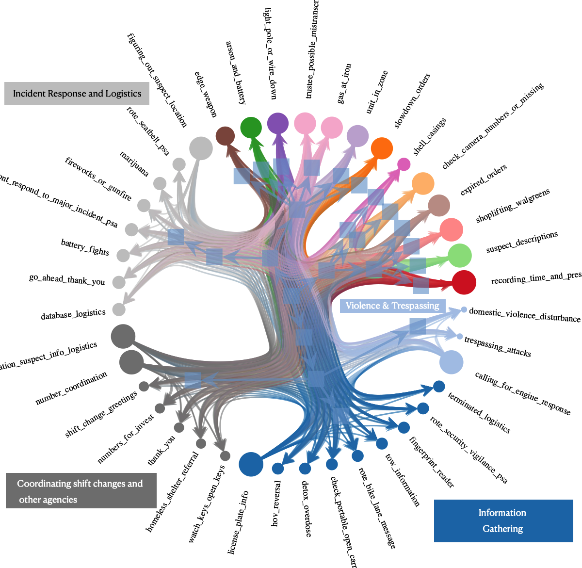
These results can be explored and improved upon, but it’s quickly clear that lots of logistical topics go together (where are the suspects, where were the gunshots, other incident response), some urgent actions go together (domestic violence, trespassing, calling for a fire engine), and some meta-conversation about shift changes and calling other agencies like referrals to a homeless shelter go together. There’s certainly some signal being captured here, and identifying it may help with classifying the broadest levels of police behavior.

Conclusion

Everything above lays the groundwork for studying police radio: gathering audio, processing it, and building tools for pattern-finding. Now it is possible to pursue the social questions we opened with and more. What can this data source reveal about policing, and how it changes over time, by region, and by demographics? The research has only just begun.